Introduction to the Online SuperLearner
Antoine Chambaz and Frank Blaauw
OnlineSuperLearner.rmdIn this guide we present a basic example of how the OnlineSuperLearner (OSL) can be used. The goal of OSL is to be able to make predictions and do inference based on (in machine learning terms) online machine learning algorithtms. The OSL can for example be used on time series data. In order to do so, it estimates a density function for each of the covariates of interest, the treatment variables of interest, and the outcome of interest. After these densities are fitted, OSL can simulate interventions and determine the outcome given such an intervention. This package relies heavily on the condensier package.
In this guide we will present a basic overview of the steps needed to perform a simulation study or to use the OSL with your own data set. We will start by installing and configuring the package. The next step is to approximate our true parameter of interest given the simulation data. This approximated truth is used as ground truth for the rest of the algorithm. Note that this step is only possible in simulation studies; in real life the true parameter of interest is not available. After approximating the parameter of interest, the next step is to perform the actual machine learning procedure. We estimate the densities and run an iteritative sampling method, in which we apply the same treatment as in the approximation step. If everything goes well, both parameters should converge to approximately the same values. Note that this guide does not apply any TMLE. We do perform an initial one-step estimation procedure, but this procedure is still in its infancy.
In this tutorial / guide we assume that the user’s working directory is the root folder of the OnlineSuperLearner repository. We also assume that the latest version of R is installed (3.4.3 at the time of writing). Also note that you can create an R file of this document by running the following command (in the root of the OnlineSuperLearner repo):
Install dependencies
Before anything else we need to install several dependencies. Most dependencies are used by OSL and some are used by Condensier. In this guide we’re using the latest (v 3.4.3 at the time of writing) version of R.
Firstly we need to install several system libraries installed: - libnlopt-dev - libcurl4-openssl-dev
Then appart from the system libraries, we need to install the R dependencies. We created a script that can be ran to install the packages needed by the online super learner. Note that running this script should not be necessary, as installing the OSL should automatically install these dependencies for you. However, it can be useful in some cases (e.g., in docker this layer can be cached). The script can be ran as follows:
An other option to install the dependencies is to install the OnlineSuperLearner package as a whole, installing all of its dependencies automatically. After installing the packages we then need to load them. We do not assume that you have installed the latest version of the OSL package, and as such will use the latest version from github:
## Removing package from '/Library/Frameworks/R.framework/Versions/3.5/Resources/library'
## (as 'lib' is unspecified)
## Downloading GitHub repo frbl/onlinesuperlearner@master
## from URL https://api.github.com/repos/frbl/onlinesuperlearner/zipball/master## Installing OnlineSuperLearner## '/Library/Frameworks/R.framework/Resources/bin/R' --no-site-file \
## --no-environ --no-save --no-restore --quiet CMD INSTALL \
## '/private/var/folders/m0/9g4fl3416h71h9j472z160f80000gn/T/Rtmp8WrGLZ/devtoolsc76a3feadfce/frbl-OnlineSuperLearner-8730f08' \
## --library='/Library/Frameworks/R.framework/Versions/3.5/Resources/library' \
## --install-tests## ## Loading required package: R6## Warning: replacing previous import 'R.utils::extract' by
## 'magrittr::extract' when loading 'OnlineSuperLearner'## Warning: replacing previous import 'magrittr::equals' by 'R.oo::equals'
## when loading 'OnlineSuperLearner'## OnlineSuperLearner## The OnlineSuperLearner package is still in beta testing. Interpret results with caution.Quick check if the correct functions are exported:
##  [1] "fit.OnlineSuperLearner"
##  [2] "PreProcessor"
##  [3] "Evaluation.log_likelihood_loss"
##  [4] "PreProcessor.generate_bounds"
##  [5] "OutputPlotGenerator.create_density_plot"
##  [6] "ConstrainedGlm.predict"
##  [7] "Simulator.GAD"
##  [8] "ML.randomForest"
##  [9] "ConstrainedGlm.fit"
## [10] ".__T__$<-:base"
## [11] ".__T__|:base"
## [12] "OutputPlotGenerator.create_training_curve"
## [13] "OutputPlotGenerator.store_oos_osl_difference"
## [14] "ML.SVM"
## [15] "InterventionParser.valid_intervention"
## [16] "Evaluation.root_mean_squared_error"
## [17] "CrossValidationRiskCalculator"
## [18] "OnlineSuperLearner"
## [19] "InterventionEffectCalculator"
## [20] "Evaluation.mse_loss"
## [21] "Data.Static"
## [22] "Evaluation.log_loss"
## [23] "OutputPlotGenerator.create_convergence_plot"
## [24] "ML.NeuralNet"
## [25] "OutputPlotGenerator.create_risk_plot"
## [26] ".__T__c:base"
## [27] ".__T__$:base"
## [28] ".__T__[<-:base"
## [29] ".__T__[:base"
## [30] "H2O.Available"
## [31] "Simulator.RunningExample"
## [32] "Data.Base"
## [33] "SMGFactory"
## [34] "Evaluation.accuracy"
## [35] "SMG.Mock"
## [36] "ConstrainedGlm.fit_new_glm"
## [37] "ConstrainedGlm.update_glm"
## [38] "Data.Stream"
## [39] "SMG.Mean"
## [40] "InterventionParser.parse_intervention"
## [41] "sampledata"
## [42] "summary.OnlineSuperLearner"
## [43] "SummaryMeasureGenerator"
## [44] "Data.Stream.Simulator"
## [45] "H2O.Initializer"
## [46] "Evaluation.mean_squared_error"
## [47] "OutputPlotGenerator.get_colors"
## [48] "OutputPlotGenerator.get_simple_colors"
## [49] "InterventionParser.is_current_node_treatment"
## [50] ".__T__length:base"
## [51] ".__T__&:base"
## [52] ".__T__[[<-:base"
## [53] "OutputPlotGenerator.export_key_value"
## [54] "RelevantVariable"
## [55] "DensityEstimation.are_all_estimators_online"
## [56] "SMG.Base"
## [57] "RelevantVariable.find_ordering"
## [58] "SMG.Lag"
## [59] "LibraryFactory"
## [60] "SMG.Latest.Entry"
## [61] "InterventionParser.first_intervention"
## [62] "Evaluation.get_evaluation_function"
## [63] "InterventionParser.generate_intervention"
Configuration
The next step is to configure several parameters for the estimation procedure itself. These meta-parameters determine how the OSL will actually learn from a very applied point of view. There are several options to configure:
-
log: Whether or not we want logging of the application. Logging can be done using theR.utilsverbose object, e.g.:log <- Arguments$getVerbose(-8, timestamp=TRUE). -
condensier_options: The options to pass to the condensier package. -
cores: The number of cores used by OSL
Apart from these very high-level settings, there are some other settings one needs to specify prior to starting the learning process:
-
training_set_size: OSL trains the estimator on a number of training examples. After that it evaluates its performance on a different (test) set. -
max_iterations: OSL will process the trainingset iteratively. That is, it won’t use all data in one go, but will use micro batches forn amax_iterationsnumber of steps. -
test_set_size: the size of the testset to use. Each iteration the algorithms are tested against a subset of the data (the testset). The size of this set can be specified using this parameter. Note that the size should be \(>= 1\), and depending on the number of algorithms \(K\), it should be \(>= K - 1\). -
mini_batch_size: for training the OSL can use a single observation (online learning) or a minibatch of observations (use \(n \ll N\) observations for learning). The size of this set can be set in themini_batch_sizeparameter. Note that this has to be >= 1 +test_set_size(one observation used for training, one for testing).
Implemented in R this looks as follows:
  library('magrittr')
  # Set the seed
  set.seed(12345)

  # Set some functions, for readability
  expit = plogis
  logit = qlogis

  # Do logging?
  log <- FALSE

  # How many cores would we like to use?
  cores = parallel::detectCores()

  # Number of items we have in our training set
  training_set_size <- 200

  # Number of items we have in our testset
  test_set_size <- 2

  # Number of iterations we want to use (this is for the online training part)
  max_iterations <- 3

  # Size of the mini batch
  mini_batch_size <- 3

  # The calculator for estimating the risk. This is just used for testing.
  cv_risk_calculator <- CrossValidationRiskCalculator$new()
Now the basic configuration for the OSL is done, we can go ahead and specify which intervention we are interested in. Interventions are specified as an R list with three elements:
-
when: When should the intervention be done? (i.e., at what time \(t\)) -
what: What should be the intervention we are doing? (e.g., set treatment to \(x \in \{0,1\}\)) -
variable: Which variable do we consider the intervention variable? (\(A\) in the TL literature)
We could also specify a list of interventions, but for now this will do. Specify the intervention as follows:
  # Number of iterations for approximation of the true parameter of interest
  B <- 1e2

  # The intervention we are interested in (intervene at time 2, give intervention 1, on variable A)
  intervention  <- list(when = c(2), what = c(1), variable = 'A')

  # The time of the outcome we are interested in
  tau <- 2
Simulation
In order to have some data to use for testing, we have to create a simulator. This simulator uses the simulation scheme as defined in CH. 8 of Blaauw (2018). For this scheme we can define various things for each of the data generating systems:
-
stochMech: the mechanism we use to generate the observations -
param: the number of steps \(t\) the mechanism is connected to the past -
rgen: the mechanism for generating the observations
For example:
  complicated_treatment <- FALSE

  # Our covariate definition
  llW <- list(
    stochMech=function(numberOfBlocks) {
      rnorm(numberOfBlocks, 0, 10)
    },
    param=c(0, 0.5, -0.25, 0.1),
    rgen=identity
  )

  # The treatment mechanism
  llA <- list(
    stochMech=function(ww) {
      rbinom(length(ww), 1, expit(ww))
    },
    param=c(-0.1, 0.1, 0.25),
    rgen=function(xx, delta=0.05){
      probability <- delta+(1-2*delta)*expit(xx)
      rbinom(length(xx), 1, probability)
    }
  )

  # The outcome variable
  if (complicated_treatment) {
      rgenfunction = function(AW){
        aa <- AW[, "A"]
        ww <- AW[, grep("[^A]", colnames(AW))]
        mu <- aa*(0.4-0.2*sin(ww)+0.05*ww) + (1-aa)*(0.2+0.1*cos(ww)-0.03*ww)
        rnorm(length(mu), mu, sd=0.1)
      }
  } else {
        rgenfunction = function(AW){
        aa <- AW[, "A"]
        mu <- 19 + aa*(0.9) + (1-aa)*(0.3)
        rnorm(length(mu), mu, sd=0.1)
      }
  }
  llY <- list(rgen = rgenfunction)
Now, using these mechanisms we need to setup our simulator. First we define the ‘truth’, or in our case, an approximation of the true parameter of interest. This parameter specifies what we expect to receive if we would run the earlier specified intervention
  # Create the simulator
  simulator  <- Simulator.GAD$new()

  # Approximate the truth under the treatment
  result.approx <- parallel::mclapply(seq(B), function(bb) {
    when <- max(intervention$when)
    data.int <- simulator$simulateWAY(
      tau,
      qw = llW,
      ga = llA,
      Qy = llY,
      intervention = intervention,
      verbose = log
    )
    data.int$Y[tau]
  }, mc.cores = cores) %>%
    unlist

  # Calculate the approximation of the true parameter of interest
  psi.approx <- mean(result.approx)

  print(psi.approx)
## [1] 19.8933The next step is to use the mechanisms to create a test set of data. Store the result so we can use it later
The OnlineSuperLearner initialization
Now everything is set-up, we can start our super learner procedure. First let’s choose a set of algorithms we wish to include in our learner. Note that OSL automatically creates a grid of learners based on te hyperparameters provided in the setup.
  algos <- list()

  algos <- append(algos, list(list(algorithm = "ML.NeuralNet",
                                  params = list(nbins = c(5), online = TRUE))))

  algos <- append(algos, list(list(algorithm = "ML.SpeedGLMSGD",
                                  params = list(nbins = c(5), online = TRUE))))
The next step is to define our relevant variables. In this example we only consider the default variables \(W\), \(A\), and \(Y\). Each of them is univariate, and the \(A\) variable is a binary variable:
  W <- RelevantVariable$new(formula = W ~ Y_lag_1 + A_lag_1 +  W_lag_1 + Y_lag_2, family = 'gaussian')
  A <- RelevantVariable$new(formula = A ~ W + Y_lag_1 + A_lag_1 + W_lag_1, family = 'binomial')
  Y <- RelevantVariable$new(formula = Y ~ A + W, family = 'gaussian')

  variable_of_interest <- Y
  relevantVariables <- c(W, A, Y)
Note the special notation for the lagged variables and the running mean variables. In the background we use the so-called SummaryMeasureGenerator, a class that automatically parses these formulae and generates the data accordingly. The idea is that given the definition provided in the previous code block, we have to generate several variables (e.g. the lags). Currently several options are provided:
-
*A*_lag_*B*: The lag operator. This will generate a lagged version of relevant variable*A*(replace with your own variable name), of lag*B*(replace with an integer, specifying the lag to use). -
*A*_mean: The running mean operator. This will generate a running mean version of relevant variable*A*(replace with your own variable name).
The last step is to actually run and fit our SuperLearner and calculate its cross-validated risk. We use the loglikelihood loss function as general loss function. Note that for this to work properly, we have to normalize our data. This is done by providing the normalize = TRUE argument to the fit function.
osl  <- fit.OnlineSuperLearner(
  formulae = relevantVariables,
  data = data.train,
  algorithms = algos,
  verbose = log,

  test_set_size = test_set_size,
  initial_data_size = training_set_size / 2,
  max_iterations = max_iterations,
  mini_batch_size = (training_set_size / 2) / max_iterations
)
## Create_risk_plot plotting to: tmp/performance_iteration_0.pdf## Create_risk_plot plotting to: tmp/performance_iteration_1.pdf## Create_risk_plot plotting to: tmp/performance_iteration_2.pdfIn order to see how well it can estimate we first generate our data set we want to use for testing as follows:
- Draw B observations from our
simulatorobject. - Input one of these observations in our algorithm.
- Sample iteratively, and set a treatment using a prespecified
variable,when, andthen. - Record the outcome of our variable of interest (\(Y\)) at time tau and we denormalize it (converting it back to the original data format).
- Repeat this procedure a large number of \(B\) times
- Finally we take the average over all \(B\) observations, giving us our estimation of the parameter of interest.
  # Should we run in parallel?
  do_parallel <- FALSE

  # Would we like to have the results of the discrete (TRUE) or continuous (FALSE) osl?
  discrete = TRUE

  interventionEffectCalculator <- InterventionEffectCalculator$new(
    bootstrap_iterations = B,
    outcome_variable = 'Y',
    parallel = do_parallel
  )

  ## Generate a block from the initial data
  osl$get_summary_measure_generator$set_trajectories(data = Data.Static$new(dataset = data.test))
## $traj_1
## <Data.Static>
## Inherits from: <Data.Base>
## Public:
## clone: function (deep = FALSE)
## get_all: active binding
## get_currentrow: active binding
## get_length: active binding
## get_remaining_length: active binding
## getNext: function ()
## getNextN: function (n = 1)
## initialize: function (dataset = NULL, url = NULL, verbose = FALSE)
## reset: active binding
## Private:
## currentrow: 1
## dataset: data.table, data.frame
## increase_pointer: function (n = 1)
## read_data_from_url: function (url)
## verbose: FALSE data_test_full <- osl$get_summary_measure_generator$getNext(1)$traj_1
result <- interventionEffectCalculator$evaluate_single_intervention(
osl = osl,
initial_data = data_test_full,
intervention = intervention,
tau = tau,
discrete = discrete
)
result %<>% unlistFinally, we can see how well the algorithms converge and estimate the approximated truth. The following plot shows this convergence for both the approximation (i.e., truth, black), and the estimation (red).
  # Calculate psi
  psi.estimation <- mean(result)

  # Plot the convergence
  y1 <- cumsum(result.approx)/seq(along=result.approx)
  y2 <- cumsum(result)/seq(along=result)

  plot(y1, ylim=range(c(y1,y2)))
  par(new=TRUE)
  plot(y2, ylim=range(c(y1,y2)), col="red", axes = FALSE, xlab = "", ylab = "")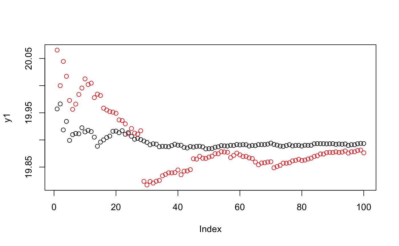
  # Print the outcome
  outcome <- paste(
    'We have approximated psi as', psi.approx,
    'our estimate is', psi.estimation,
    'which is a difference of:', abs(psi.approx - psi.estimation)
  )
  print(outcome)
## [1] "We have approximated psi as 19.8932989285089 our estimate is 19.8762323582572 which is a difference of: 0.0170665702516928"The result should be something like:
[1] "We have approximated psi as 19.9016316150146 our estimate is 19.9018591048906 which is a difference of: 0.000227489875989306"Prediction and sampling
Apart from calculating a variable of interest, the online superlearner package also offers the functionality to predict the probability of a given outcome (conditionally on other variables), and to sample conditionally on a set of variables. The package offers two S3 methods to do so: predict and sample.
Examples of both methods are listed below
  # Predict some variables for our Y outcome variable. The newdata can be a data.table:
  predict(osl, data.test, Y = Y)
## $`ML.NeuralNet-vanilla.nbins-5_online-TRUE`
## W A Y
## 1: 0.047656893000 0.3931003230 1.7185446639
## 2: 0.008368826782 0.2037153541 1.1693212812
## 3: 0.083819944570 0.3931003230 2.2036386657
## 4: 0.139103313378 0.6068996770 4.2432198934
## 5: 0.008368795848 0.2038907987 2.6469346727
## ---
## 994: 0.009412959418 0.3931003230 0.4302204738
## 995: 0.009412959418 0.3931003230 0.5021638134
## 996: 0.083819944570 0.6068996770 1.2173643100
## 997: 0.013161352358 0.6068996770 1.2607557515
## 998: 0.013972004366 0.2033905454 1.2265829733
##
## $`ML.SpeedGLMSGD-vanilla.nbins-5_online-TRUE`
## W A Y
## 1: 0.00395228053929672 0.4471364328 3.1019177980
## 2: 0.02221178539600475 0.5233270896 1.1707741285
## 3: 0.02587857647378037 0.4308073398 2.5925366166
## 4: 0.04267507827893337 0.4345088912 4.5540838241
## 5: 0.01561972953089770 0.5188321510 1.5118474539
## ---
## 994: 0.01738160876121666 0.6037654894 0.4695156837
## 995: 0.04536158131858053 0.8182840411 0.5629124447
## 996: 0.23432258597802774 0.3809454203 1.2294078480
## 997: 0.01234977603177382 0.5721809027 1.2820427338
## 998: 0.00000001029352521 0.3536386026 1.2406165215
##
## $osl.estimator
## Y
## 1: 2.8034306194
## 2: 1.1704606510
## 3: 2.5086250173
## 4: 4.4870094424
## 5: 1.7567625625
## ---
## 994: 0.4610370483
## 995: 0.5498048549
## 996: 1.2268092420
## 997: 1.2774496915
## 998: 1.2375885357
##
## $dosl.estimator
## Y
## 1: 1.7185446639
## 2: 1.1693212812
## 3: 2.2036386657
## 4: 4.2432198934
## 5: 2.6469346727
## ---
## 994: 0.4302204738
## 995: 0.5021638134
## 996: 1.2173643100
## 997: 1.2607557515
## 998: 1.2265829733## $`ML.NeuralNet-vanilla.nbins-5_online-TRUE`
## W A Y
## 1: 2.729799644261 1 19.87342119
## 2: 2.539940838993 1 19.38256540
## 3: 11.562932189113 0 20.05892690
## 4: 2.028798272006 1 19.31183775
## 5: 0.008400103984 1 19.39875417
## ---
## 994: 6.360187833376 0 19.58764240
## 995: 13.376053325041 1 19.83707358
## 996: 4.731774960868 0 19.09163024
## 997: -1.395993451743 0 19.33553360
## 998: -4.519055774431 1 19.30621830
##
## $`ML.SpeedGLMSGD-vanilla.nbins-5_online-TRUE`
## W A Y
## 1: 11.73011806904 0 20.06252635
## 2: -4.02036382814 1 19.11880059
## 3: 2.79541757241 1 19.98294067
## 4: -3.79616612418 1 19.71746617
## 5: 5.44557527225 0 19.57374404
## ---
## 994: 0.05465629624 1 19.97427923
## 995: 1.97766003074 1 19.98552443
## 996: -0.41456301980 1 19.30640988
## 997: 2.41114456563 0 19.33765272
## 998: -2.89544691271 1 19.34497146
##
## $osl.estimator
## Y
## 1: 20.02172357
## 2: 19.17571251
## 3: 19.99933604
## 4: 19.62994468
## 5: 19.53598689
## ---
## 994: 19.89085551
## 995: 19.95349354
## 996: 19.26006738
## 997: 19.33719548
## 998: 19.33660978
##
## $dosl.estimator
## Y
## 1: 19.87342119
## 2: 19.38256540
## 3: 20.05892690
## 4: 19.31183775
## 5: 19.39875417
## ---
## 994: 19.58764240
## 995: 19.83707358
## 996: 19.09163024
## 997: 19.33553360
## 998: 19.30621830These methods return the predicted probabilities and sampled data for each of the algorithms in a list (thus a list of data.table objects). If instead of these functions the actual R6 functions are used, the result is slightly different, and might be useful to discuss. The result of the R6 methods is a list with two entries: normalized and denormalized. The normalized entry contains the result normalized according to the preprocessor that had been defined based on the initial data frame. The denormalized entry contains the data in its original form (i.e., the normalization has been undone). Generally only the latter is of interest. These entries (the normalized and denormalized entry) again contain a number of lists, each with an outcome for each of the candidate estimators.